WRF-Solar® EPS
The WRF-Solar® model (Jimenez et al. 2016) is a specific configuration and augmentation of the Weather Research and Forecasting (WRF) model. Previous efforts have been largely devoted to enhance the aerosol-cloud-radiation physics. To extend the WRF-Solar capabilities beyond deterministic forecasts, we are developing the WRF-Solar Ensemble Prediction System (WRF-Solar EPS).
WRF-Solar EPS introduces stochastic perturbations in the most relevant variables for solar irradiance forecasts. The variables have been identified with tangent linear models of selected parameterizations (Yang et al. 2020). The model provides a user-friendly configuration to set the characteristics of the perturbations for each variable (in an ascii configuration file) and to select the variables to perturb (in the WRF namelist).
A beta version of the WRF-Solar EPS model is available.
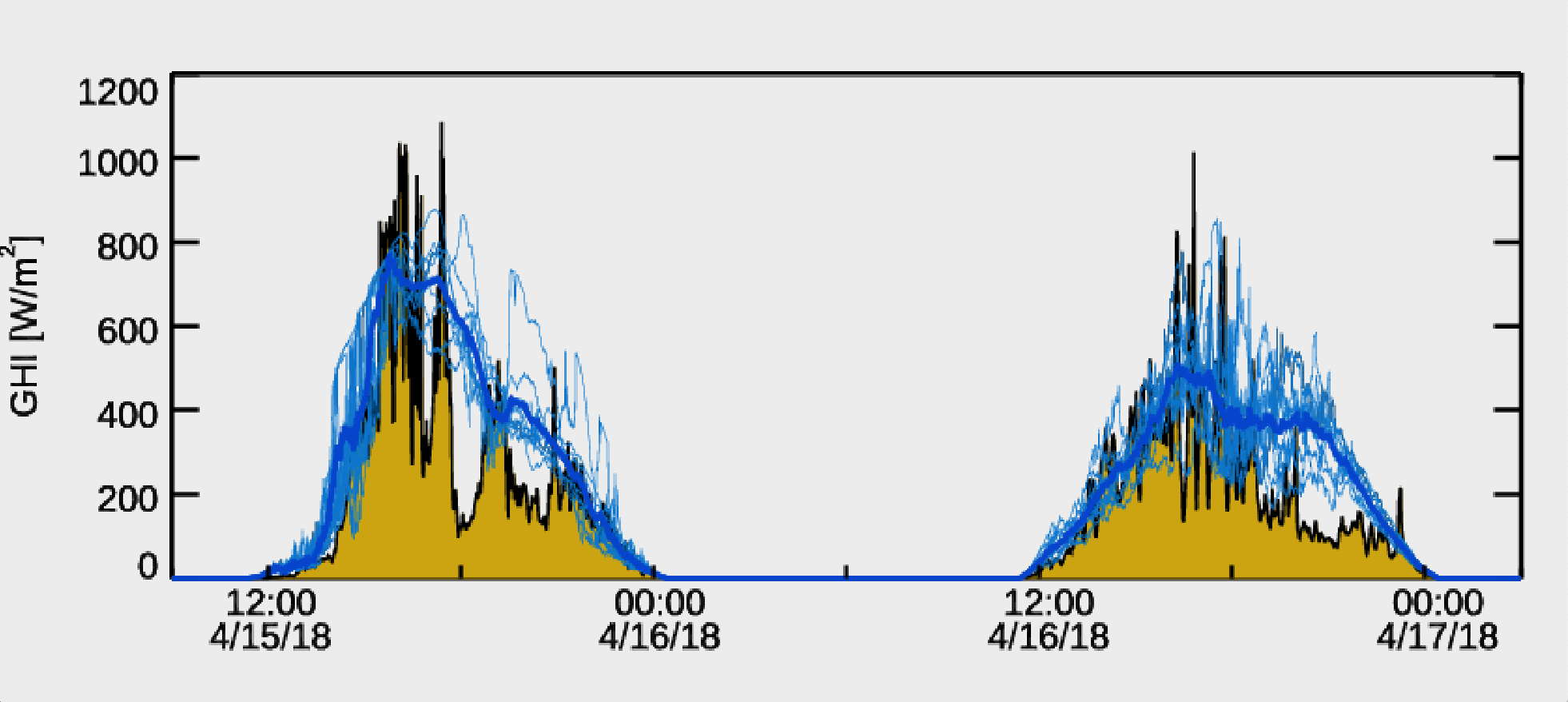
Global horizontal irradiance forecast as a function of the lead time: thin lines) WRF-Solar EPS ensemble members, thicker line) ensemble mean. Observations are also shown (shaded).
References
Jimenez, P. A., J. P. Hacker, J. Dudhia, S. E. Haupt, J. A. Ruiz-Arias, C. A. Gueymard, G. Thompson, T. Eidhammer and A. Deng, 2016a: WRF-Solar: Description and Clear-Sky Assessment of an Augmented NWP Model for Solar Power Prediction. Bull. Amer. Met. Soc., 97, 1249-1264. doi:10.1175/BAMS-D-14-00279.1
Yang, J., J. H. Kim, P. A. Jimenez, M. Sengupta, J. Dudhia, Y. Xie, A. Golnas and R. Giering, 2020: An efficient method to identify uncertainties of WRF-Solar variables in forecasting solar irradiance using a tangent linear sensitivity analysis. Solar Energy (In press)
Description
The variables to perturb were identified using six parameterizations responsible for radiation and cloud formation and dissipation:
- Thompson microphysics (Thompson et al. 2008)
- Mellor–Yamada–Nakanishi–Niino (MYNN; Nakanishi and Niino 2009) planetary boundary layer (PBL)
- Noah surface model (Noah LSM; Chen and Dudhia 2001)
- Deng shallow cumulus system (Deng et al. 2014, Jimenez et al. 2016)
- Fast-All-sky Radiation Model (FARMS) radiation (Xie et al. , 2016)
- A parameterization of the unresolved clouds module based on relative humidity (CLD3)
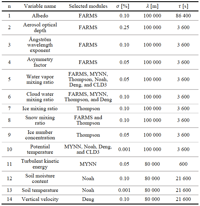
The most relevant input variables for each module were selected using tangential linear analysis. With this aim, we developed tangent linear models (TLM) for each of the selected modules. The TLMs were used to analyze uncertainties of the output variables to uncertainties in the input variables in order to select the most sensitive variables controlling radiative transfer and cloud processes. We identified 14 variables (Yang et al. 2020): surface albedo, aerosol optical depth, Ångström exponent, asymmetry factor, water vapor mixing ratio, cloud/ice/snow mixing ratios, ice number concentration, potential temperature, turbulent kinetic energy, soil moisture content, soil temperature, and vertical velocity. Table 1 shows a complete list of these variables (column 2) and their associated parameterizations (column 3).
Table 1 also shows the characteristics of the stochastic perturbations (columns, 4, 5 and 6). The perturbations are obtained through sampling an isotropic Gaussian distribution. The perturbations are characterized by the standard deviation of the Gaussian distribution (σ, column 4), the wavelength (λ, column 5), and the decorrelation time (τ, column 6) between consecutive perturbations (Berner et al. 2009 and Jankov et al. 2017). WRF-Solar EPS adds the stochastic perturbations inside each parameterization every model time step.
Table 1. Characteristics of the 14 stochastic perturbations in WRF-Solar EPS.
References
Berner, J., G. Shutts, M. Leutbecher, and T. Palmer, 2009: A spectral stochastic kinetic energy backscatter scheme and its impact on flow-dependent predictability in the ECMWF en- semble prediction system. J. Atmos. Sci., 66, 603–626.
Chen, F., and J. Dudhia, 2001: Coupling an advanced land surface-hydrology model with the Penn State-NCAR MM5 modeling system. Part I: Model implementation and sensitivity, Mon. Weather Rev.,129, 569–585.
Deng, A., B. J. Gaudet, J. Dudhia, and K. Alapaty, 2014: Implementation and evaluation of a new shallow convection scheme in WRF. 26th Conf. on Weather Analysis and Forecasting/22nd Conf. on Numerical Weather Prediction, Atlanta, GA, Amer. Meteor. Soc., 12.5. [Available online at https:// ams.confex.com/ams/94Annual/webprogram/Paper236925.html.]
Jankov, I., and Coauthors, 2017: A performance comparison between multiphysics and stochastic approaches within a North American RAP ensemble. Mon. Wea. Rev., 145, 1161–1179.
Jimenez, P.A., S. Alessandrini, S. E. Haupt, A. Deng, B. Kosovic, J. A. Lee, L. Delle Monache, 2016: The role of unresolved clouds on short-range global horizontal irradiance predictability. Mon. Wea. Rev., 144, 3099 - 3107. doi:10.1175/MWR-D-16-0104.1.
Nakanishi, M., and H. Niino, 2009: Development of an improved turbulence closure model for the atmospheric boundary layer. J. Meteor. Soc. Japan, 87, 895–912.
Thompson, G., P. R. Field, R. M. Rasmussen, and W. D. Hall, 2008: Explicit forecasts of winter precipitation using an improved bulk mi- crophysics scheme. Part II: Implementation of a new snow parameterization. Mon. Wea. Rev., 136, 5095–5115.
Xie, Y., M. Sengupta, and J. Dudhia, 2016: A Fast All-sky Radiation Model for Solar applications (FARMS): Algorithm and performance evaluation. Sol. Energy, 135, 435-445.
Yang, J., J. H. Kim, P. A. Jimenez, M. Sengupta, J. Dudhia, Y. Xie, A. Golnas and R. Giering, 2020: An efficient method to identify uncertainties of WRF-Solar variables in forecasting solar irradiance using a tangent linear sensitivity analysis. Solar Energy (In press.)
User's guide
WRF-Solar EPS requires to describe the characteristic of the stochastic perturbations for each variable and to select the variables to perturb. These two steps are summarized as follows:
- The STOCHPERT.TBL file in the run directory is used to set the characteristics of the perturbations. The file has one row for each variable (14 variables). The columns correspond to the variable number, the standard deviation of the perturbation (in %), the wave length (in meters), the decorrelation time (in seconds), the maximum value of standard deviations allowed in the amplitude of the perturbation, the random seed used to generate the sequence of random numbers, and the dimension of each variables (0 for 2D, and 1 for 3D)
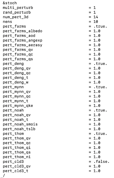
- The ‘$stoch’ block in the WRF namelist is used to set the variables to perturb. Setting ‘multi_perturb’ to 1 activates the perturbations. The variable ‘nens’ is the # of the ensemble member and determines the random number sequence in the simulation. The user also needs to select which parameterization (logical flag) and which variables (0.0 off and 1.0 on), will be perturbed. The example below activates the perturbations in all variables of all parameterizations except for CLD3.

Publications
Yang, J., J.H. Kim, P.A. Jimenez, M. Sengupta, J. Dudhia, Y. Xie, A. Golnas and R. Giering, 2020: An efficient method to identify uncertainties of WRF-Solar variables in forecasting solar irradiance using a tangent linear sensitivity analysis. Solar Energy (In press.)
Yang, J., Sengupta, M., Xie, Y., Jimenez, P.A. and Kim, J.H., 2019. Adjoint Sensitivity of FARMS to the Forecasting Variables of WRF-Solar. In 36th European Photovoltaic Solar Energy Conference and Exhibition.
Kim, J.H., Jimenez, P.A., Dudhia, J., Yang, J., Sengupta, M., Xie, Y., 2020, “Probabilistic Forecast of All-sky Solar Radiation Using Enhanced WRF-Solar”, In 37th European Photovoltaic Solar Energy Conference and Exhibition.
Contact
Please direct questions/comments about this page to:
Pedro Jimenez Munoz
Proj Scientist III

